1 Introduction
This is a summary of the tests performed in the Spring of 2019 to quantify the impact of variable seeing on the quality of the Differential Chromatic Refraction (DCR) correction algorithm, as initially described in DMTN-037. The current state of the DCR algorithm makes the simplifying assumption that all of the input exposures used to construct the template have identical PSFs, and there has been some concern that the quality of the model will degrade when those input exposures have variable seeing. In this note I compare the performance of templates created with DcrAssembleCoaddTask with our current standard, CompareWarpAssembleCoaddTask, and estimate the range of observing conditions where the current algorithm is sufficient.
2 Simulations
To compare the two algorithms, I first generated a large set of simulated observations with a progressively increasing range of seeing. Observing conditions were drawn from an OpSim run using the feature-based scheduler [1], with the requirement that the selected field have eight observations in one year, and at least one observation taken at airmass greater than 1.15 [2]. The observing conditions for the field used for this analysis are listed in Table 1 below.
| Visit | Airmass | Parallactic Angle | Seeing |
|---|---|---|---|
| 1010000 | 1.018 | 180° | 0.876” |
| 1010001 | 1.035 | 0° | 0.620” |
| 1010002 | 1.102 | 180° | 1.219” |
| 1010003 | 1.044 | 180° | 0.611” |
| 1010004 | 1.952 | 180° | 0.941” |
| 1010005 | 1.174 | 0° | 0.634” |
| 1010006 | 1.065 | 180° | 0.600” |
| 1010007 | 1.125 | 0° | 0.745” |
From these input observing conditions, nine sets of eight simulated images were created using StarFast, each with a different range of allowed seeing. The control set of eight observations forced the seeing of each image to be equal to that of the best seeing image, while the successive sets allowed the range of seeing to increase by 10% from the last set. In each case, the original distribution of seeing values was scaled so that the minimum and maximum values matched those given in Table 2 below, rather than clipping values outside the bounds.
| Run # | Seeing range |
|---|---|
| 1 | 0.60” - 0.60” |
| 2 | 0.60” - 0.66” |
| 3 | 0.60” - 0.73” |
| 4 | 0.60” - 0.80” |
| 5 | 0.60” - 0.88” |
| 6 | 0.60” - 0.97” |
| 7 | 0.60” - 1.06” |
| 8 | 0.60” - 1.17” |
| 9 | 0.60” - 1.29” |
The images from each simulation run were coadded using both CompareWarpAssembleCoaddTask and DcrAssembleCoaddTask, resulting in 18 different templates for the tests. To make the tests directly comparable, the same set of 24 simulated science images were used for image differencing with each of the 18 templates. The observing conditions for the science images were taken unmodified from OpSim, and covered a wide range of airmasses and seeing values (Table 3).
| Visit | Airmass | Parallactic angle | Seeing |
|---|---|---|---|
| 2010000 | 1.043 | 180° | 0.623” |
| 2010001 | 1.128 | 180° | 0.884” |
| 2010002 | 1.189 | 0° | 0.766” |
| 2010003 | 1.515 | 180° | 0.943” |
| 2010004 | 1.175 | 0° | 0.742” |
| 2010005 | 1.093 | 0° | 0.871” |
| 2010006 | 1.186 | 0° | 1.165” |
| 2010007 | 1.066 | 180° | 0.692” |
| 2010008 | 1.037 | 0° | 0.909” |
| 2010009 | 1.198 | 180° | 0.893” |
| 2010010 | 1.052 | 0° | 0.672” |
| 2010011 | 1.261 | 0° | 0.876” |
| 2010012 | 1.090 | 180° | 0.686” |
| 2010013 | 1.044 | 180° | 1.176” |
| 2010014 | 1.944 | 180° | 1.451” |
| 2010015 | 1.042 | 180° | 0.948” |
| 2010016 | 1.118 | 0° | 0.533” |
| 2010017 | 1.188 | 180° | 0.648” |
| 2010018 | 1.091 | 0° | 0.936” |
| 2010019 | 1.680 | 180° | 1.110” |
| 2010020 | 1.043 | 0° | 1.059” |
| 2010021 | 1.069 | 0° | 1.281” |
| 2010022 | 1.032 | 180° | 0.737” |
| 2010023 | 1.115 | 0° | 1.377” |
3 Results
3.1 Deep Coadd Source Measurements
When the input exposures used to construct the DCR model have variable seeing, the sources begin to smear out. This smearing happens to some extent with CompareWarpAssembleCoaddTask as well, but because extreme values are clipped the effect is reduced. A similar clipping can’t be used in the DCR algorithm, however, because that erases real information from high airmass observations with DCR-stretched sources.
For this comparison, I ran source detection for all 18 reruns, but copied the source detection catalog from the constant seeing DCR coadd run to replace the detections for all the other runs. Thus the source measurements were performed at exactly the same locations for all runs, and in the same order. To compare different runs, I first removed any sources that were flagged in any of them. Then I normalized the aperture fluxes by dividing by the PSF flux from the constant seeing run, and took the median from all of the unflagged sources. In the figure below I plot that normalized aperture flux as a function of aperture size for several of the simulations with different seeing ranges, and for both the CompareWarp and DCR coadd algorithm.
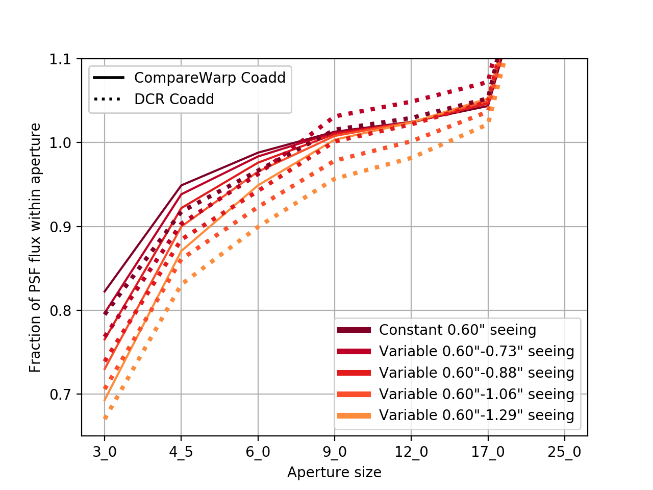
Figure 1 The fraction of the constant-seeing case PSF flux detected within each aperture for deep coadded images constructed with either DcrAssembleCoaddTask or CompareWarpAssembleCoaddTask, and for different ranges of seeing in the input images.
In the case of constant seeing (the darkest solid and dashed lines) the aperture flux is very similar between the two algorithms. However, as the range of seeing in the input images increases, the additional smearing of the DCR image shows up as a gradual decrease in the measured flux in each aperture. The CompareWarp-built coadds, on the other hand, maintain a constant measured flux within a nine arcsecond aperture, and closely match the PSF flux at that point. This suggests that the ratio of the nine arcsecond aperture flux to the constant-seeing PSF flux is a good metric for the loss of flux due to varying PSF widths for the DCR coadds, and this value remains close to one for seeing ranges up to 0.60” - 0.88”. Thus, as long as the PSF size of the worst seeing observation is no more than 50% greater than the size of the PSF of the best seeing observation, it should be appropriate to use DcrAssembleCoaddTask in its present form.
3.2 Image Difference Residuals
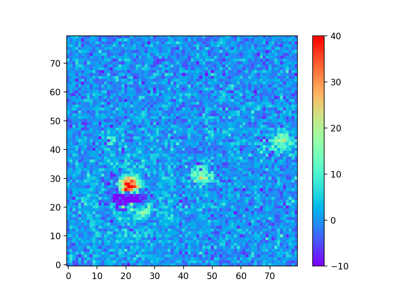
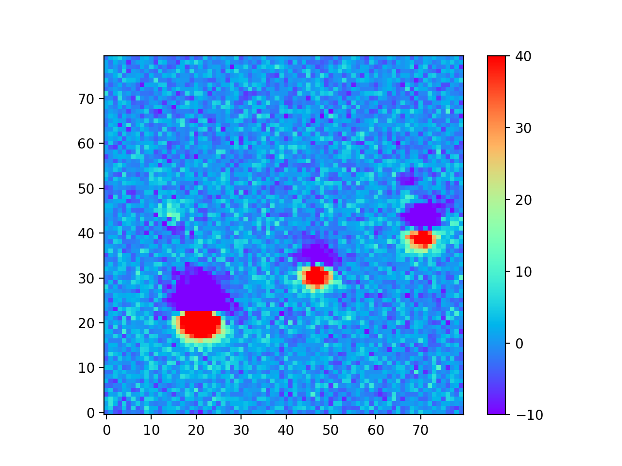
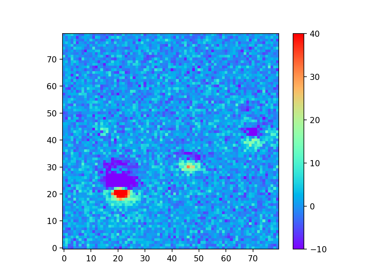
The motivation for creating the DCR model was to make better templates for image differencing, which I tested using the 24 science images from Table 3 above. In Image Difference Residuals below, I chose a small region from one science image (visit 2010011 in Table 3 above), and compare the residual images using the two algorithms and three different ranges of seeing. For observations like this one at airmasses above 1.2, the residuals are quite bad if the template is built without accounting for DCR, even in the constant seeing case. Thus, for these simulated images at least, the difference between the two types of template is much greater than the differences between any of the ranges of seeing of the input images, even for the case with the greatest variation in seeing. For image differencing, this suggests that the DCR-matched template should be used if there will be any moderate- to high-airmass observations, even if the seeing range of the input observations is highly variable. For a quantitative comparison of the two algorithms using science images with a wide range of airmasses, see Image Difference Source Detection below.
| Template seeing range | Deep coadd template | DCR-matched template |
|---|---|---|
Constant 0.60” Visit 2010011 Airmass 1.261 Seeing 0.876” |
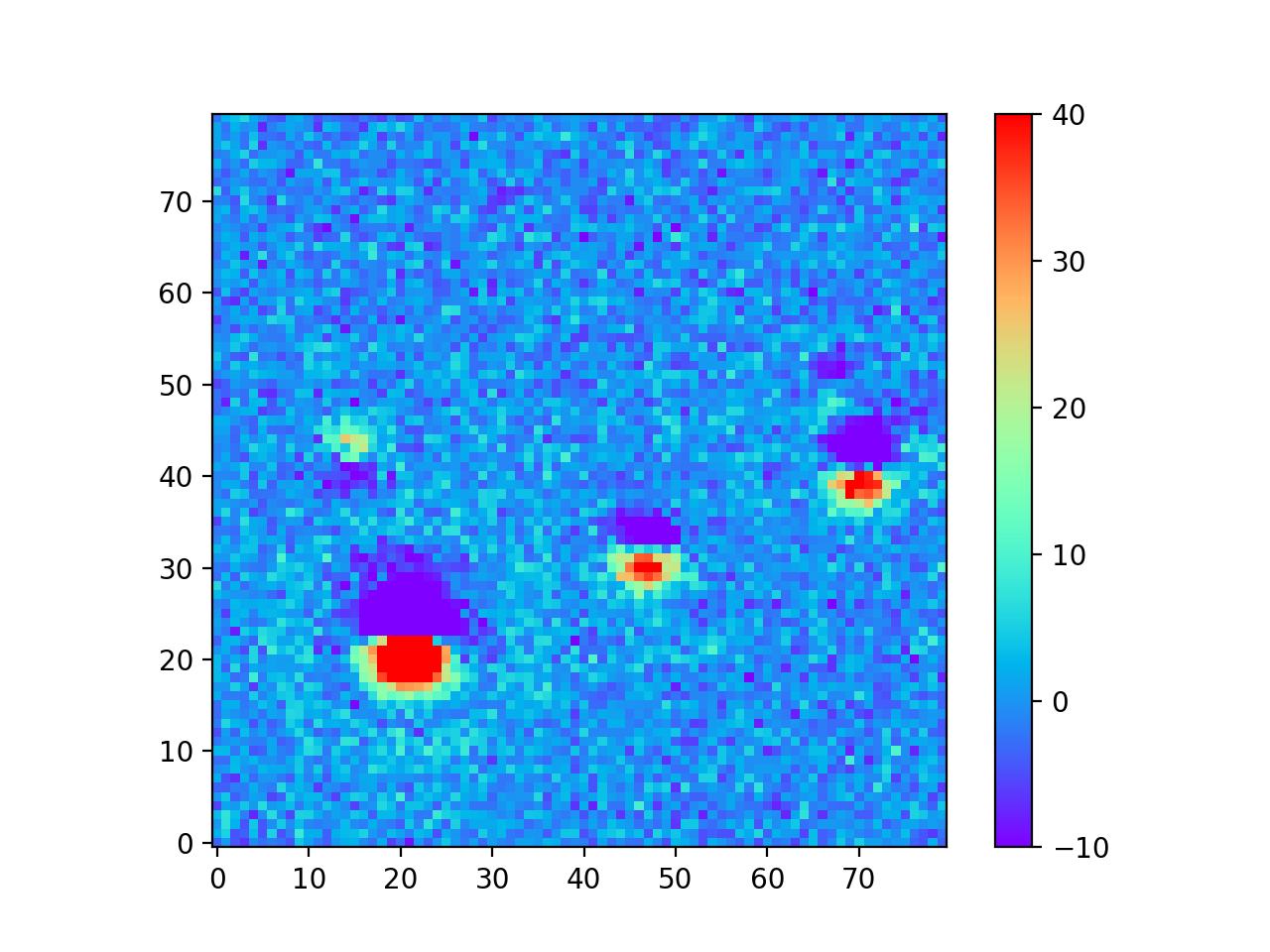
|
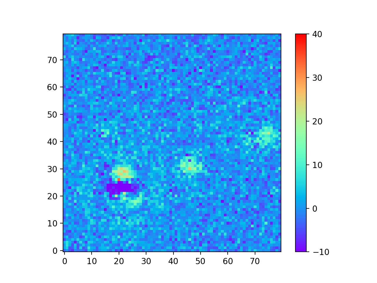
|
0.60” - 0.88” Visit 2010011 Airmass 1.261 Seeing 0.876” |
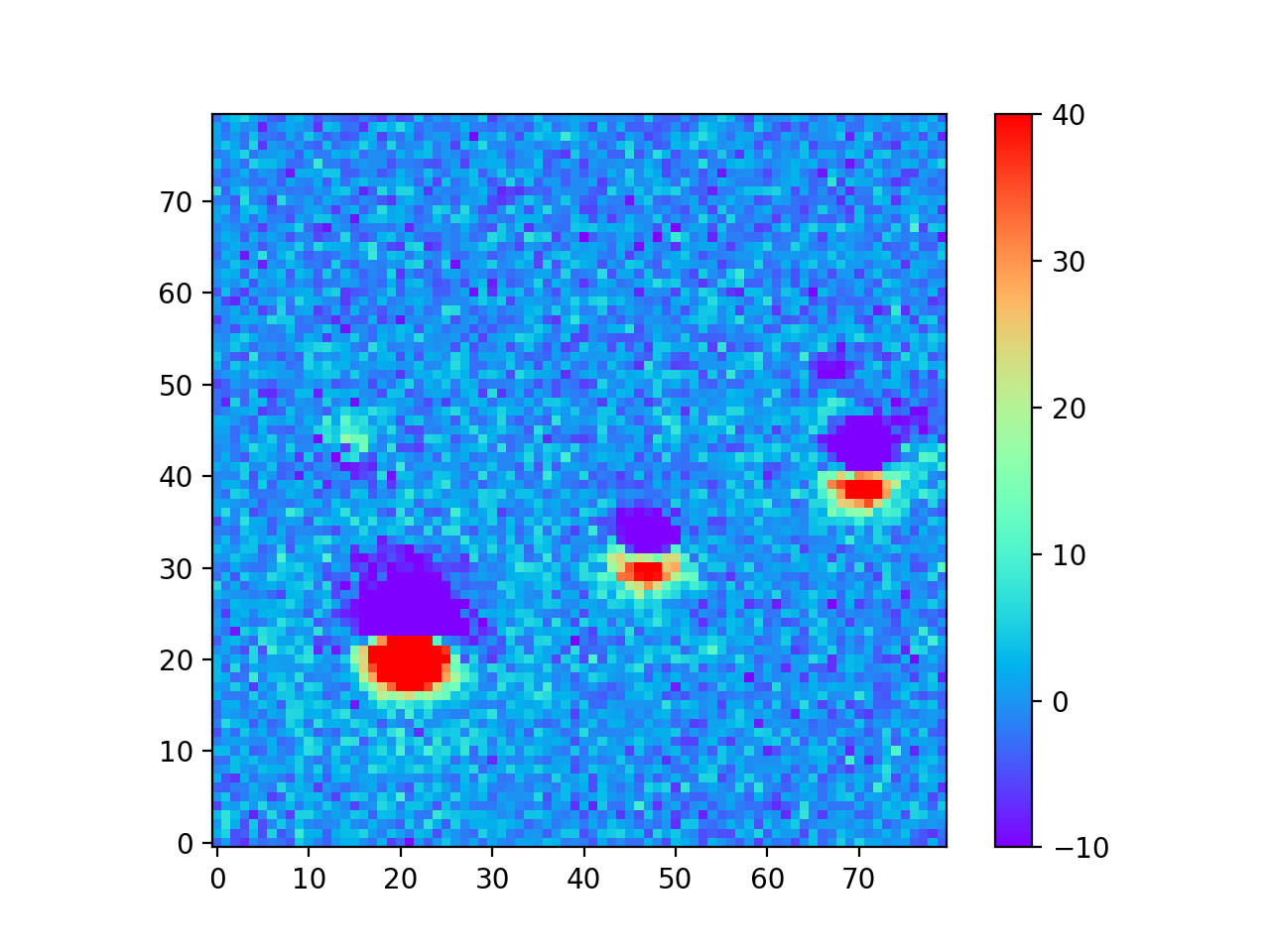
|
|
0.60” - 1.29” Visit 2010011 Airmass 1.261 Seeing 0.876” |
|
|
3.3 Image Difference Source Detection
The simulated images contained no real variable sources, so every detection in the image difference is a false detection and the fewer dipoles or other detections the better. The improved image difference residuals above correspond to an equally improved reduction in the number of detected dipoles and false detections, which are plotted below. In the plots below, the number of dipoles or sources in the image differences using CompareWarp templates is taken as the baseline, which is compared to the number of dipoles or sources in the equivalent image difference using DCR-matched templates. It is interesting to note that the reduction in the number of dipoles approaches 100% above airmass 1.2, but the reduction in the number of sources plateaus at ~80%. This captures the sources that were not well fit by either algorithm, as well as the sources that were measured as dipoles in the CompareWarp residuals but had a more complicated structure in the DCR residual.
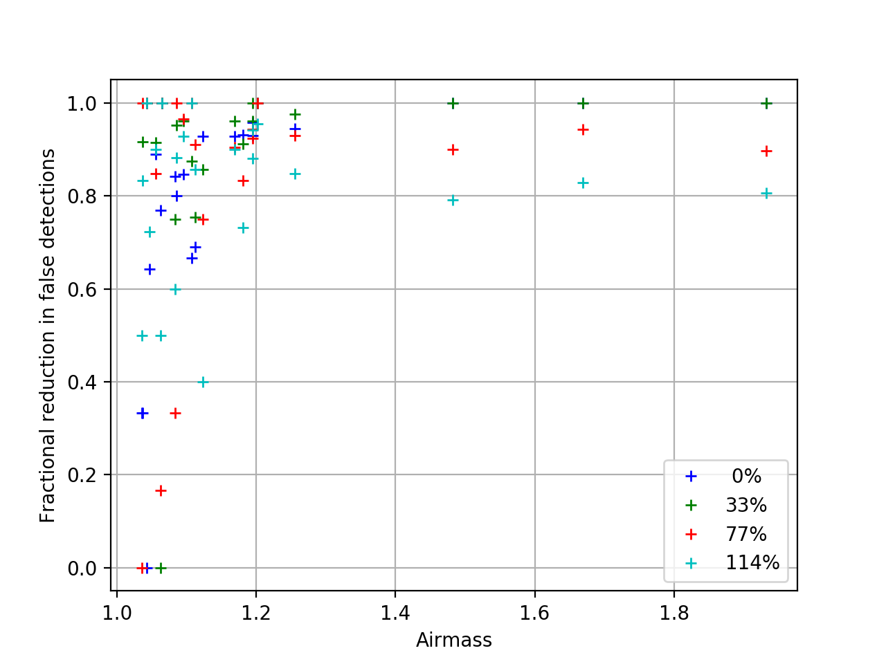
Figure 2 The reduction in the number of dipoles detected in image differences using DCR-matched templates, as a fraction of the number of dipoles in the equivalent image difference using a CompareWarp template. The colors refer to the range in seeing of the input images.
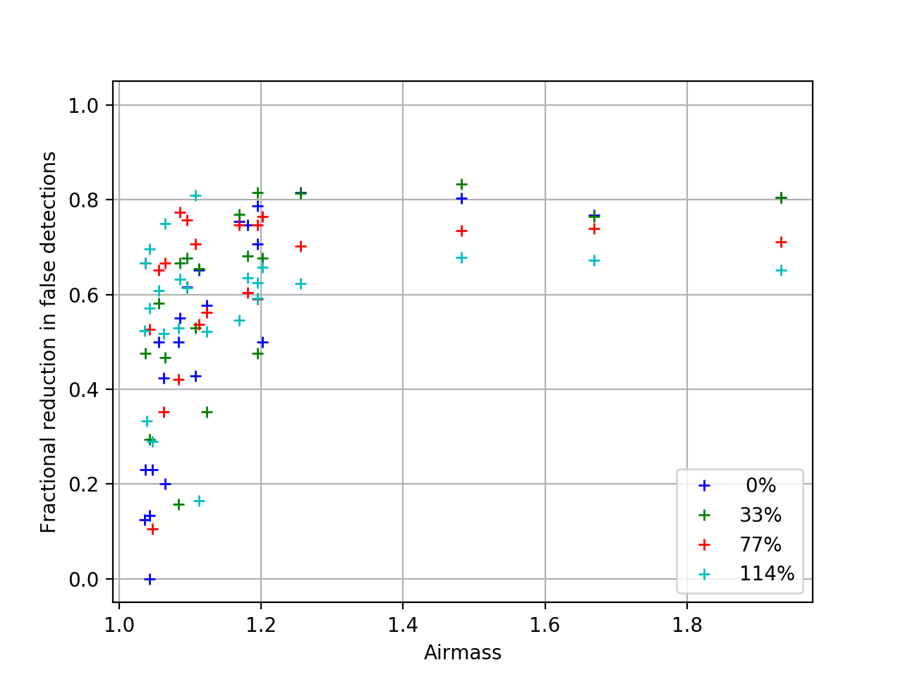
Figure 3 The reduction in the number of sources of any kind detected in image differences using DCR-matched templates, as a fraction of the number of dipoles in the equivalent image difference using a CompareWarp template. The colors refer to the range in seeing of the input images.
4 Conclusions
The DCR model generates better templates for image differencing for all ranges of seeing I tested, and has a correspondingly reduced number of false sources detected in the image difference. Above airmass 1.1, the number of false detections in these simulations was cut in half, even in the run with the largest range of seeing. This suggests that if the range of airmasses is greater than 0.1, the DCR model should be used to construct templates. A caution is that the DCR algorithm appears to lose some of the flux from sources detected on the coadd when the seeing range of the input images is above roughly 50%. If it was extended to account for variable seeing, however, that flux would be better fit and it is likely that the matched templates would be further improved.
4.1 Scheduler Implications
A typical year of LSST g-band observations is planned to include an average of 8 observations per field. The expected distribution of seeing values for those observations from OpSim ranges from 0.456” to 1.668”, with a typical value of ~0.7” as seen in Figure 4 below.
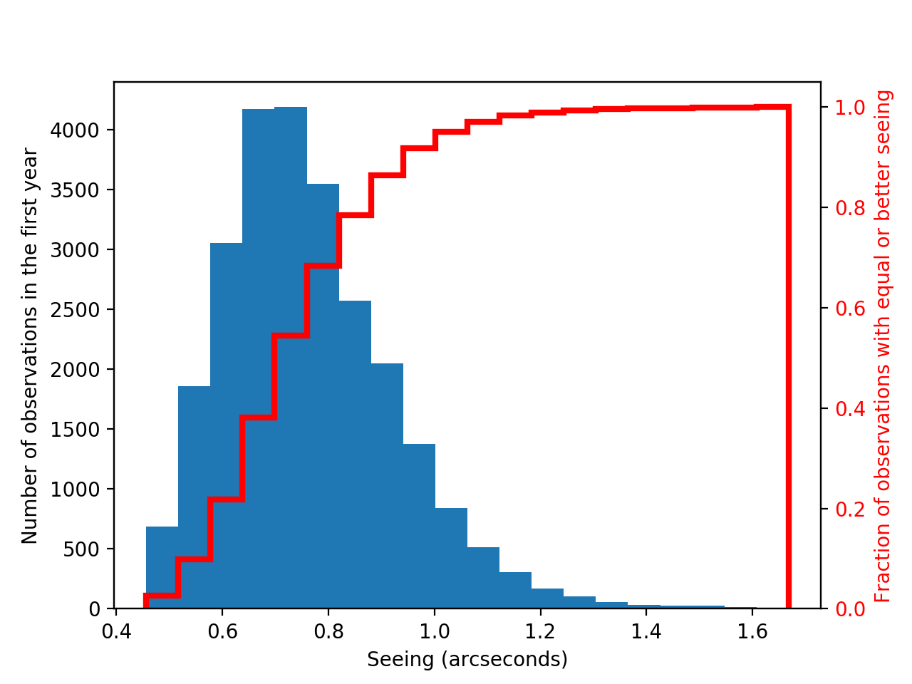
Figure 4 Histogram of seeing values for the first year of LSST g-band observations, with the cumulative distribution overplotted in red.
In order to build DCR-matched templates using just the data from the first year we need a minimum of 5 observations, with the worst seeing no more than 50% greater than the best seeing for each field. Given the expected distribution of seeing values, this means that we would need to cut exceptionally good seeing observations as well as poor ones in order to keep the ratio of the worst to the best under 50%, as found in Deep Coadd Source Measurements. In Table 5, I have computed the average number of acceptible observations we would have for a typical field given the tolerance set on that ratio of the worst to the best seeing values, and I list the associated range of seeing values.
| Seeing tolerance | Seeing range | Percent usable | Average number usable |
|---|---|---|---|
| 50% | 0.636” - 0.954” | 66.7% | 5.33 |
| 60% | 0.626” - 1.002” | 73.8% | 5.9 |
| 70% | 0.596” - 1.013” | 79.4% | 6.35 |
| 80% | 0.566” - 1.019” | 84.1% | 6.72 |
| 90% | 0.566” - 1.075” | 87.6% | 7.01 |
| 100% | 0.546” - 1.092” | 90.4% | 7.24 |
With the limitation of a 50% range of seeing, we would achieve the minimum number of 5 observations per field, but only on average. That means that many fields could be left with insufficient observations to construct DCR-matched templates from the first year of data, though there should be plenty after year 2. If we were to relax the constraint on the seeing so that the worst seeing observation of a field was allowed to be twice the best seeing (a seeing tolerance of 100% in the chart), then we would be able to use all or all but one of the observations for most fields. For image differencing, the results of Image Difference Source Detection suggest that we could use the looser tolerance with DcrAssembleCoaddTask as it is now and achieve a significant reduction in the number of dipoles and false detections. However, if we were able to include variable PSFs in the calculation of the DCR model, then we should be able to achieve that reduction without worrying about losing flux, and without having to exclude the observations with the best seeing.
| [1] | with the exception that the observations were forced to be on the local Meridian. This simplification was due to a bug discovered in the simulator that resulted in incorrect parallactic angles off the Meridian. |
| [2] | The conditions set on the number of visits and the airmass range were set to give the DCR algorithm sufficient leverage to constrain the model. |